At Target we aim to make shopping more fun and relevant for our guests through extensive use of data – and believe me, we have lots of data! Tens of millions of guests and hundreds of thousands of items lead to billions of transactions and interactions. We regularly employ a number of different machine learning techniques on such large datasets for dozens of algorithms. We are constantly looking for ways to improve speed and relevance of our algorithms and one such quest brought us to carefully evaluate matrix multiplications at scale – since that forms the bedrock for most algorithms. If we make matrix multiplication more efficient, we can speed up most of our algorithms!
Before we dig in, let me describe some properties of the landscape we will be working in. First, what do I mean by large scale? A large scale application, at a minimum, will require its computation to be spread over multiple nodes of a distributed computing environment to finish in a reasonable amount of time. These calculations will use existing data that are stored on a distributed file system that provides high-throughput access from the computing environment. Scalability, in terms of storage and compute, should grow as we add to these resources. As the system grows larger and more complex, failures will become more commonplace. Thus, software should be fault-tolerant.
Fortunately, there is a lot of existing open-source software that we can leverage to work in such an environment, particularly Apache Hadoop for storing and interacting with our data, Apache Spark as the compute engine, and both Apache Spark and Apache Mahout for applying and building distributed machine learning algorithms. There are many other tools that we can add to the mix as well, but for the purposes of this post we will limit our discussion to these three.
With that out of the way, lets dig in!
Don’t Forget the Basics
Begin with good old paper and pencil. Yeah, I know this is about large scale matrix operations that you could never do by hand, but the value in starting with a few examples that you can work out with pencil and paper is indispensable.
- Make up a few matrices with different shapes - maybe one square and nonsymmetric, one square and symmetric, and one not square.
- Choose the dimensions such that you can perform matrix multiplication with some combination of these matrices.
- Work out the results of different operations, such as the product of two matrices, the inverse of a matrix, the transpose, etc.
There is no need to go overboard with this. It can all fit on a single piece of paper, front and back maximum.
Test the Basics
Now it’s time to start making use of Spark and Mahout, and the best place to begin is by implementing the examples you just worked out by hand. This has two obvious purposes:
- You can easily verify that you are using the packages correctly. i.e. Your code compiles and runs.
- You can easily verify that what you have calculated at runtime is correct.
What is nice about these two simple things, is that a lot of important concepts are unearthed just by getting this far. Particularly, how you take your initial data and transform it into a matrix type and what operations are supported.
What you will find is that there are 3 basic matrix types (in terms of distribution); the local matrix (Spark, Mahout), the row matrix (Spark, Mahout), and the block matrix (Spark). Each of these types differ in how they are initialized and how the matrix elements are distributed. Visually this is depicted for 3 different m x n matrices below:
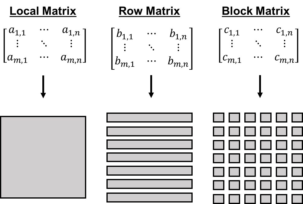
In the above figure you can think of each block as representing a portion of the matrix that is assigned to a partition. Thus, a local matrix is stored entirely on a single partition. A row matrix has its rows distributed among many partitions. And a block matrix has its submatrices distributed among many partitions. These partitions can in turn be distributed among the available executors.
What’s the takeaway? Applications that rely solely on operations on local matrices will not benefit from additional executors, and will be limited to matrices that can fit in memory. Applications that use row matrices will benefit from additional executors, but as n gets larger and larger will suffer from the same limitations as local matrices. Applications that rely solely on block matrices can scale to increasingly large values of m and n.
The caveat is that underlying algorithms increase in complexity as you move from local to row to block matrices. As such, there may not be an existing pure block matrix implementation of the algorithm you wish to use, or the algorithm may feature a step that multiplies a row matrix by a local matrix. Understanding the implementation details from this perspective can help you to anticipate where the bottlenecks will be as you attempt to scale out.
From Basics to the Big Leagues
At this stage we aim to ramp up from operations on small matrices to operations on larger and larger matrices. To do this, we begin by sampling our real data down to a small size. Using this sample data we can benchmark the performance of the matrix operations we are interested in. Then, we move to a larger sample size and repeat the benchmarking process. In this way, we can ramp up to the problem size of interest, while building and developing intuition about the resources required at each new scale.
In benchmarking performance, there are basically 3 parameters that we can play with:
- The number of executors.
- The amount of executor memory.
- The number of partitions that we decompose our distributed matrices into.
There are other parameters we could consider, such as the number of cores per executor. But these 3 will serve as a very useful starting point.
Number of Executors
We can hone in on the number of executors to use based on a strong scaling analysis. For this analysis, we run our calculation with our sample data using p executors and record the time. We then repeat the exact same calculation with the same sample data but now use 2p executors and record the time. We can repeat this process, increasing the number of executors by a factor of 2 each time. Ideally, we would hope to find that every time we double the number of executors our calculation completes in half the time, but in practice this will not be the case. The additional complexity of the distributed algorithms and communication cost among partitions will result in a performance penalty, and at some point during this process it will no longer be “worth it” to pay this penalty. This is shown in the figure below:
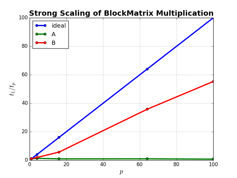
In the above figure we show strong scaling for the multiplication of two square block matrices. The x-axis represents the number of cores used in a carrying out the multiplication. The y-axis represents scalability, defined as the amount of time it takes to complete the calculation on a single core divided by the amount of time it takes to complete the same calculation using p cores. The blue curve represents ideal strong scaling as discussed above. The green curve represents the product C = A*A, and the red curve represents D = B*B. Matrix A fits comfortably in memory on a single core, and Matrix B is two orders of magnitude larger than A. What is apparent is that there is little to no benefit of parallelism in calculating the product C. Whereas, for the larger product, D, we observe a nearly linear speedup up to 100 cores.
We can decide if it is “worth it” more concretely by setting a threshold for efficiency, defined as the ratio of the observed speedup versus the ideal speedup. A fair value for the efficiency threshold could be in the range of 50 to 75 percent. Higher than this is perhaps unrealistic in many cases, and lower is probably wasteful, as extra resources are tied up but not sufficiently utilized.
Executor Memory
We can think about the executor memory in two different ways. One option, in terms of performance, is that we desire to have enough executor memory such that we avoid any operations spilling to disk. A second option, in terms of viability, is to assess whether or not there is enough executor memory available to perform a calculation, regardless of how long it takes.
It is helpful to try to find both of these limits. Begin with some value of executor memory. Monitor the Spark UI to detect if data is spilling to disk. If it is, rerun with double the executor memory until it no longer does. This can represent the optimal performance case. For the viability option rerun while reducing the executor memory by a factor of 2 until out of memory exceptions won’t allow the calculation to complete. This will give you a nice bounds on what is possible versus what is optimal.
Number of Partitions
A final parameter for tuning that we will consider here is the number of partitions that we decompose our distributed matrices into. As a lower limit, you want the number of partitions to match the default parallelism (num-executors * executor-cores), else there will be resources that are completely idle. However, in practice, the number of partitions should be the default parallelism multiplied by some integer factor, perhaps somewhere between 2 to 5 times is an optimal range. This is known as overdecomposition, and helps reduce the idle time of executors by overlapping communication and computation.
In fact, we could overdecompose by much larger factors, but we would see that the performance degrades. This is because the benefit of overlapping communication with computation is now less than the overhead of the compute engine managing all of the different partitions. However, if we are aiming for viability instead of performance this may be the only way to proceed. Increasing the number of partitions will reduce the memory footprint of each partition, allowing them to be swapped to and from disk as needed.
Performance Tips
As you ramp up to larger and larger problem sizes performance will become more and more critical. I have found that simply adjusting some spark configuration settings can give a significant boost in performance:
- Serialization concerns the byte representation of data and plays a critical role in performance of Spark applications. The
KryoSerializercan offer improved performance with a little extra work:spark.serializer=org.apache.spark.serializer.KryoSerializer. See here for more info on serialization. - If you notice long periods of garbage collection, try switching to a concurrent collector:
spark.executor.extraJavaOptions="-XX:+UseConcMarkSweepGC -XX:+UseParNewGC". I have found this to be a nice reference on garbage collection. - If you notice stages that are spending a lot of time on the final few tasks then speculation may help:
spark.speculation=true. Spark will identify tasks that are taking longer than normal to complete and assign copies of these tasks to different executors, using the result that completes first.
Wrapping Up
It is fair to think that this process is tedious, and that there is a lot to digest, but the intuition and knowledge developed will serve you as you continue to work with these tools. You should be able to short-circuit this process and enter at the ramp up stage, beginning with a relatively modest sample size. Your experience will guide you in selecting a good estimate for the initial amount of resources and you can continue to tune and ramp up from there.
If you found this interesting then you may be interested in some of the projects that we are working on at our Pittsburgh location. We have positions available for data scientists and engineers and a brand new office opening in the city’s vibrant Strip District neighborhood.
About the Author
Patrick Pisciuneri is a Lead Data Scientist and part of Target’s Data Sciences team based in Target’s Pittsburgh office.